A Browser-Native Reformulation of Dynamical EBSD Simulation
A browser-native reformulation of dynamical EBSD
Dynamical electron backscatter diffraction (EBSD) simulation has traditionally meant local native software (for example EMsoftOO workflows) or vendor machines. This project takes a different route: a browser-native master-pattern simulator built on a low-rank Lyapunov reformulation of the dynamical scattering problem, running entirely in WebGPU with no install and no server round-trip.
What a master pattern is, and why it is expensive
A dynamical EBSD master pattern is the backscattered intensity a crystal emits as a function of exit direction, integrated over the depth the electrons sample and over the energy they lose on the way out. The “dynamical” part is the catch: backscattered electrons re-diffract many times before they leave, so the intensity in any direction is the solution of a strongly coupled multi-beam problem rather than a single kinematical structure factor.
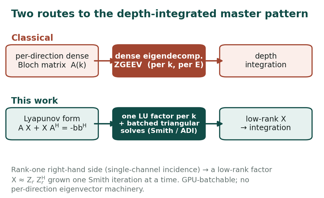
The classical recipe handles this one direction at a time. For each incident/exit direction \(\mathbf{k}\) you build a dense Bloch-wave dynamical matrix \(A(\mathbf{k})\), take its eigendecomposition (the ZGEEV-style path), and propagate the eigenmodes through depth, repeating the whole thing for every energy bin. Eigendecomposition is the bottleneck: it is cubic in the number of beams, it has to be redone for every direction and every energy, and it maps poorly onto a GPU.
The reformulation: a Lyapunov equation with a rank-one source
The key observation is that the quantity we actually need — the depth-integrated mode coupling — is the solution \(X\) of a Lyapunov matrix equation
\[ A X + X A^{\mathsf H} = -\,\mathbf{b}\,\mathbf{b}^{\mathsf H}, \]
where the right-hand side is rank one, because a master pattern is excited by single-channel incidence (one beam in). A rank-one source is exactly the regime where Lyapunov solutions are well approximated by a low-rank factor \(X \approx Z_r Z_r^{\mathsf H}\) with \(Z_r\) having only a handful of columns. So instead of asking for every eigenmode, we ask for a low-rank object that already is the depth-integrated answer.
The reason this reformulation works for EBSD is that the Monte Carlo depth profiles coming from David C. Joy’s model are, for nearly every incident angle, crystal, and voltage between 5 and 40 kV that I checked, very closely approximated by exponential decay curves. Once the depth weight is effectively exponential, the depth integral lands naturally in this Lyapunov form.
To my knowledge this is the first time the low-rank Lyapunov reformulation has been applied to electron-diffraction master-pattern synthesis.
The LU solver
The low-rank factor is built with a Smith-type iteration (a single-shift ADI recurrence; in the Cayley-transform view each step applies a Cayley map of \(A\)). Per direction, you form the shifted operator and compute one LU factorization \(A_{\text{shift}} = LU\). Each Smith iteration is then a pair of triangular solves against that stored \(L\) and \(U\) — no re-factoring, no eigenvectors — appending one block of columns to the low-rank factor \(Z_r\). The number of iterations is the rank \(r\).
A batched LU factorization followed by many batched triangular solves is a good fit for the GPU: thousands of directions share the same kernel, the work is regular, and runtime scales with the number of low-rank steps rather than with dense eigenvector machinery. The LU factorize/solve kernels live in the underlying WasmGPU compute engine; the fix that made the factor/solve numerically robust is the piece this post ships. Before 2026-06-07 there was a bug in those LU kernels that only showed up once the matrices got past roughly 100x100, so small test problems could look fine while the larger production cases did not.
Choosing the rank
The rank \(r\) is the one knob that matters.
![]()
A few things fall out of this that are worth stating plainly:
- The band network is low-rank-friendly. Even at rank 1 the Kikuchi bands — the dominant structure of the pattern — are already in the right places with the right widths. Setting the rank to about 3 gives a very plausible master pattern across most of the hemisphere.
- Zone axes are the holdout. Near low-index zone axes many bands cross, the dynamical coupling is strongest, and the low-rank approximation converges slowest. Those directions need a higher rank to reach full intensity.
- Extra rank mostly just brightens. Past the point where the bands are resolved, each additional Smith iteration largely adds a brightness halo around the zone axes rather than new structure.
Right now every direction runs to the same fixed rank, which keeps the kernels simple and the batch regular. The better answer is a per-direction residual check that stops early where the solve has already converged and keeps iterating near the zone axes — I just haven’t written those kernels yet.
Other approaches I tried
A few other things I tried first before Smith iteration:
- Extended and rational Krylov methods for the Lyapunov solve. Strong convergence per iteration, but the basis bookkeeping and orthogonalization fit GPU batching far worse than plain LU + solves.
- Arnoldi / rational-Krylov bases, including sharing a single basis across neighboring \(\mathbf{k}\) vectors to amortize the build. In practice the shared basis was never quite good enough for the directions that needed it most (again, the zone axes).
- Newton–Schulz iterations for the full-rank solution. They converge quadratically and are matrix-multiply-shaped, but they target the dense solution, which throws away the rank-one structure that makes the problem cheap.
Controls
- CIF parsing with editable site-level thermal (B-iso) terms.
- Beam and truncation controls: voltage, sigma, dmin, Lambert half-width, Bethe thresholds, chunk size, and energy-bin width.
- Symmetry-aware north/south hemisphere viewing.
- NPZ export of the integrated outputs.
Current limitations and next steps
This is an active research implementation. The biggest open item, besides the early-stopping kernels above: the ML surrogate that replaces Monte Carlo depth profiling still has known errors (for example, Forsterite shows an incorrect marginal and needs retraining), and more benchmarking is needed for both speed and numerical accuracy across materials and parameter ranges.
Try it
Open the app, pick a preset (for example Ni), keep the defaults, and press Run. Then sweep dmin and the Bethe cutoffs to watch pattern detail and runtime trade off against each other.